Quantcast
Channel: Getting Started – PROC-X.com
Viewing all 68 articles
Browse latest View live

Create a SAS macro variable that contains a list of values

$
0
0

Parameters in SAS procedures are specified a list of values that you manually type into the procedure syntax. For example, if you want to specify a list of percentile values in PROC UNIVARIATE, you need to type the values into the PCTLPTS= option as follows: proc univariate data=sashelp.cars noprint; var […]

The post Create a SAS macro variable that contains a list of values appeared first on The DO Loop.


What is a moving average?

$
0
0

A moving average (also called a rolling average) is a satistical technique that is used to smooth a time series. Moving averages are used in finance, economics, and quality control. You can overlay a moving average curve on a time series to visualize how each value compares to a rolling […]

The post What is a moving average? appeared first on The DO Loop.

Group processing in SAS: The NOTSORTED option

$
0
0

Novice SAS programmers quickly learn the advantages of using PROC SORT to sort data, followed by a BY-group analysis of the sorted data. A typical example is to analyze demographic data by state or by ZIP code. A BY statement enables you to produce multiple analyses from a single procedure […]

The post Group processing in SAS: The NOTSORTED option appeared first on The DO Loop.

Read data into vectors or into a matrix: Which is better?

$
0
0

In the SAS/IML language, you can read data from a SAS data set into a set of vectors (each with their own name) or into a single matrix. Beginning programmers might wonder about the advantages of each approach. When should you read data into vectors? When should you read data […]

The post Read data into vectors or into a matrix: Which is better? appeared first on The DO Loop.

Create dummy variables in SAS

$
0
0

A dummy variable (also known as indicator variable) is a numeric variable that indicates the presence or absence of some level of a categorical variable. The word "dummy" does not imply that these variables are not smart. Rather, dummy variables serve as a substitute or a proxy for a categorical […]

The post Create dummy variables in SAS appeared first on The DO Loop.

Save descriptive statistics for multiple variables in a SAS data set

$
0
0

Descriptive univariate statistics are the foundation of data analysis. Before you create a statistical model for new data, you should examine descriptive univariate statistics such as the mean, standard deviation, quantiles, and the number of nonmissing observations. In SAS, there is an easy way to create a data set that […]

The post Save descriptive statistics for multiple variables in a SAS data set appeared first on The DO Loop.

Create a package in SAS/IML

$
0
0

This post was kindly contributed by The DO Loop - go there to comment and to read the full post.

In a previous post I showed how to download, install, and use packages in SAS/IML 14.1. SAS/IML packages incorporate source files, documentation, data sets, and sample programs into a ZIP file. The PACKAGE statement enables you to install, uninstall, and manage packages. You can load functions and data into your current IML session and thereby leverage the work of the experts who wrote the package.

Do you have some awesome SAS/IML functions to share? Are you an expert in some subject area? This article describes how to create a SAS/IML package for others to use.


Share knowledge: Create a package in #SAS/IML
Click To Tweet


The following list shows the main steps to create a SAS/IML package. Each step is demonstrated by using the polygon package that I created for the paper “Writing Packages: A New Way to Distribute and Use SAS/IML Programs.”
You can download the polygon package and examine its files and structure.

1. Create a root-level directory

The first step is to think of a name for your SAS/IML package. The
name must be a valid SAS name, which means it must contain 32 characters or less, begin with a letter or underscore,
and contain only letters, underscores, and digits.
Create a directory that has this name in all lowercase letters. For example, the root-level directory for the polygon package is named polygon.

2. Create the info.txt file in the root-level directory

The info.txt file is a manifest. It provides information about the names of the source files in the package. It consists of a series of keyword-value pairs. The SAS/IML User’s Guide provides complete details about the form of the info.txt file, but an example file follows:

# SAS/IML Package Information File Format 1.0
Name:        polygon
Description: Computational geometry for polygons
Author:      Rick Wicklin <Rick.Wicklin@sas.com>
Version:     1.0
RequiresIML: 14.1
SourceFiles: PolyArea.iml
             PolyCentroid.iml
             PolyDraw.iml
             <...list additional files...>

The first line of the
info.txt file specifies the file format. Use exactly the line shown here.
The value of the Name keyword specifies the name of the package. When you create a ZIP file (Step 6), be sure to match the case exactly.

3. Create the source files

For most SAS/IML packages, the functionality is provided by a series of related functions. Put all source files in the source subdirectory.

A source file usually contains one or more module definitions. The source files cannot contain the PROC IML statement or the QUIT statement because those statement would cause an IML session to exit when the source file is read. Source files are read in the order in which they are specified in the info.txt file.

I like to put each major function in its own source file, although sometimes I include associated helper function in the same file.
I begin function names with a short prefix that identifies the package to which the functions belong. For example, most functions in the polygon package begin with the prefix “POLY”. Internal-only functions (that it, those that are not publically documented) in the package begin with the prefix “_POLY”.

I like to use “.iml” as a file extension to remind me that these are snippets of IML programs. However, you can use “.sas” as an extension if you prefer.

4. Document the SAS/IML package

Even if your package is very useful, people won’t want to use it if there isn’t sufficient documentation about how to use it. You can provide two kinds of documentation. The main documentation is usually a PDF file in the help subdirectory. You might also include slideshows, Word documents, or any other useful files. The secondary documentation is a plain (ASCII) text file that has the same name as your package. For example, the polygon package contains the file
polygon.txt in the help subdirectory. This file is echoed to the SAS log when a user installs the package and then submits the PACKAGE HELP polygon statement.

5. Create other files and subdirectories

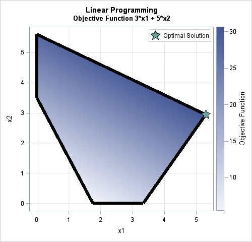
Sometimes the best way to show someone how to use a package is to write a driver program that loads the package, calls the functions, and displays the results. Driver programs and other sample programs should be put in the programs subdirectory.

For the polygon package, I included the file Example.sas, which shows how to load the package and call each function in the package. I also included other programs that test the functions. For example, the drawing function (POLYDRAW) has many options, so I wanted to show how to use each option. I also show how to define and use non-simple polygons, which are polygons that have edge intersection.

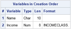
Another sure-fire way to make sure that users know how to use your functions is to include sample data.
If you have data sets to distribute, create a subdirectory named data. You can put SAS data sets, CSV files, and other sources of data into that directory.

If you have other files to distribute, create additional subdirectories. For example, you might have a C directory if you include C files or an R subdirectory if you include R files.

6. Create a ZIP file

At this point, the directories and files for the polygon package looks like the following:

C:%HOMEPATH%My DocumentsMy SAS Filespolygon
|   info.txt
|
+---data
|   simple.sas7bdat, states48.sas7bdat
|
+---help
|   polygon.docx, polygon.pdf, polygon.txt
|
+---programs
|   Example.sas, TestNonSimplePoly.sas, TestPolyDraw.sas, TestPolyPtInside.sas
|
---source
    PolyArea.iml, PolyBoundingBox.iml, PolyCentroid.iml, ..., PolyRegular.iml

The last step is to run a compression utility to create a ZIP file that contains the root-level directory and all subdirectories. The name of the ZIP file should match the package name, including the case. For example, the ZIP file for the polygon package is named polygon.zip. The following image shows creating a ZIP file by using the WinZip utility. Other popular (and free) alternatives are 7-Zip, PeaZip, and PKZip.

Creating a ZIP file for a SAS/IML Package

7. Test and upload your package

Your SAS/IML package is now ready to be tested. Make sure that you can successfully use the PACKAGE INSTALL, PACKAGE LOAD, and PACKAGE HELP statements on your package. If you are distributing data sets, test the PACKAGE LIBNAME statement.

When you are satisfied that the package installs and loads correctly, you can share the package with others. To share your work in-house, ask your system administrator to load the package into the PUBLIC collection so that everyone in your workgroup can use it. If you want to make the package available to others outside of your company, upload the package the SAS/IML File Exchange. You can follow the directions in the article “How to contribute to the SAS/IML File Exchange.”

Summary

Creating a package is a convenient way to share your work with others in your company or around the world. It enables other SAS/IML programmers to leverage your expertise and programming skills. And who knows, it just might make you famous!

For complete details about how to create a package, see the “Packages” chapter of the SAS/IML User’s Guide.

tags: Getting Started, Packages

The post Create a package in SAS/IML appeared first on The DO Loop.

This post was kindly contributed by The DO Loop - go there to comment and to read the full post.

How to fit a variety of logistic regression models in SAS

$
0
0

This post was kindly contributed by The DO Loop - go there to comment and to read the full post.

SAS software can fit many different kinds of regression models. In fact a common question on the SAS Support Communities is “how do I fit a <name> regression model in SAS?”
And within that category,
the most frequent questions involve how to fit various logistic regression models in SAS.

There are many types of logistic regression models:

  • The traditional logistic model has a binary (or binomial) response variable.
  • Well-known extensions of the logistic model include ordinal regression (for an ordinal response) and multinomial regression (for a discrete but unordered response).
  • Special models handle situations such as repeated measures (longitudinal data) or random effects.
  • Other models include conditional logistic regression, survey logistic regression, Bayesian logistic regression, and fractional logistic regression (which gets the Coolest Name Award).

If you know the procedure that you want to use, you can read the procedure documentation and follow the examples to perform the analyses.
In practice, however, you might know the reverse information: You know the analysis that you want to perform, but you do not know which SAS procedure implements that regression model.

I was therefore pleased to discover a short SAS Knowledge Base article titled “Types of logistic (or logit) models that can be fit using SAS.”
This article provides a “reverse look-up”: Given the type of logistic regression model that you want to fit, it provides the name of the SAS procedures that support that analysis!


Logistic models that can be fit with SAS: A reverse look-up resource. #SAStip
Click To Tweet


Use this resource the next time you need to know which SAS procedure can conduct a certain variant of logistic regression.
Bookmark it, print it out, tattoo it on your forearm, or come to my blog and type “HOW TO FIT A LOGISTIC MODEL” into the search box. But don’t forget it!
This resource is a treasure for the SAS statistical programmer.

tags: Getting Started, Statistical Programming

The post How to fit a variety of logistic regression models in SAS appeared first on The DO Loop.

This post was kindly contributed by The DO Loop - go there to comment and to read the full post.

Grids and linear subspaces

$
0
0

This post was kindly contributed by The DO Loop - go there to comment and to read the full post.

parallelepiped

A grid is a set of evenly spaced points. You can use SAS to create a grid of points on an interval, in a rectangular region in the plane, or even in higher-dimensional regions like the parallelepiped shown at the left, which is generated by three vectors. You can use vectors, matrices, and functions in the
SAS/IML language to obtain a grid in a parallelepiped.

Evenly spaced points in an interval

In one dimension, you can use a DO loop in the SAS DATA step to construct evenly spaced points in an interval.
In the SAS/IML language, you can construct a vector of evenly spaced values operation without writing a DO loop. You can use the DO function, or you can use the colon operator (which SAS/IML documentation calls the “index creation operator“). The results are equivalent, as shown in the following program:

proc iml;
a = 2; b = 5; N = 5;
delta = (b-a) / N;
y = do(a, b, delta);    /* Method 1: DO function: start=1, stop=b, step=delta */
x = a +  delta*(0:N);   /* Method 2: Use colon operator and vector sum */
print y, x;

span2d1

Subdivide a vector subspace

The second method generalizes to any linear subspace. For example, suppose you are given a vector u with magnitude α = ||u||. Then the following SAS/IML statements create points that are evenly spaced points along the vector u.
The magnitudes of the N vectors are 0, α/N, 2α/N, and so forth up to α.

/* linear spacing along a vector */
u = {3 2 1};
delta = u / N;         /* Note: delta is vector */
w = delta @ T(0:N);    /* i_th row is (i-1)*u */
print w;

span2d2

It’s always exciting to use the Kronecker product operator (@). The Kronecker product operator multiplies delta by 0, 1, 2, …, N and stacks the results. Notice that the ith column of the w matrix is a linear progression from 0 to the ith component of u. Each row is a vector in the same direction as u.

Grids in a linear subspace

It is only slightly harder to generate a grid of points in two or higher dimensions. In the DATA step, you can use nested DO loops to generate a grid of points in SAS. In the SAS/IML language, you can use the EXPANDGRID function.


Generate evenly spaced grid points in SAS. #SAStip
Click To Tweet


In fact, with the help of linear algebra, the EXPANDGRID function enables you to construct a grid in any linear subspace. Recall that a linear subspace is the “span,” or set of all linear combinations, of k basis vectors.

From a linear algebra perspective, a rectangular grid is a set of discrete, evenly spaced, linear combinations of the standard Cartesian basis vectors
e1,
e2, …
ek.
In a linear algebra course you learn that a matrix multiplication enables you to change to another set of basis vectors.

To give a concrete example, consider a rectangular grid of points in the square [0,1]x[0,1].
In the following SAS/IML program, the
rows of the matrix G contain the grid points. You can
think of each row as being a set of coefficients for a linear combination of the
basis vectors
e1 and
e2.
You can use those same coefficients to form linear combinations of any other basis vectors. The program shows how to form a grid in the two-dimensional linear subspace that is spanned by the vectors
u = { 3 2 1} and
v = {-3 5 2}:

h = 1/N;
/* generate linear combinations of basis vectors e1 and e2 */
G = ExpandGrid( do(0,1,h),  do(0,1,h) );  
 
u = { 3 2 1};
v = {-3 5 2};
M = u // v;      /* create matrix of new basis vectors */
grid = G * M;    /* grid = linear combinations of basis vectors u and v */

span2d

In the graph, the three-dimensional vectors u and v are indicated. The grid of points is a set of linear combinations of the form (i/N) u + (j/N) v, where 0 ≤ i, j ≤ N. The grid lies on a two-dimensional subspace spanned by u and v. The points in the grid are colored according to the values of the third component: blue points (lower left corner) correspond to low z-values whereas red points (upper right corner) correspond to high z-values.

Grids are important for visualizing multivariate functions. The function in this example is linear, but grids also enable you to visualize and understand nonlinear transformations.

tags: Getting Started, Matrix Computations

The post Grids and linear subspaces appeared first on The DO Loop.

This post was kindly contributed by The DO Loop - go there to comment and to read the full post.

The SELECT statement in the SAS DATA step

$
0
0

This post was kindly contributed by The DO Loop - go there to comment and to read the full post.

Every beginning SAS programmer learns the simple IF-THEN/ELSE statement for conditional processing in the SAS DATA step.
The basic If-THEN statement handles two cases: if a condition is true, the program does one thing, otherwise the program does something else.

Of course, you can handle more cases by using multiple ELSE IF statements.
I have seen SAS programs that contain contains dozens of ELSE clauses.
Sometimes a long sequence of IF-THEN/ELSE statements is necessary, such as when you are testing complex logical conditions.

Flow chart diagram for a switch statement (SELECT statement)

An alternative control statement in SAS is the SELECT-WHEN statement. The SELECT-WHEN statement
(sometimes simply called the SELECT statement) enables you to conditionally execute statements based on the value of a single categorical variable. Usually the variable can have three or more valid values that you want to handle.

The following example uses the Sashelp.Heart data set, which contains
data for 5,167 patients in a medical study. The Smoking_Status variable is a categorical variable that encodes the average number of cigarettes that each patient smokes per day.
The following DATA step view implements a recoding scheme, which is sometimes the easiest way to
force levels of a nominal variable to appear in a natural order during a SAS analysis.

/* example of using the SELECT statement */
data Heart / view=Heart;
set sashelp.heart;
select (Smoking_Status);
   when ('Non-smoker')        Smoking_Cat=1;
   when ('Light (1-5)')       Smoking_Cat=2;
   when ('Moderate (6-15)')   Smoking_Cat=3;
   when ('Heavy (16-25)')     Smoking_Cat=4;
   when ('Very Heavy (> 25)') Smoking_Cat=5;
   otherwise                  Smoking_Cat=.;
end;
run;

The SELECT-WHEN statement is easy to read. You specify the name of a variable on the SELECT statement.
You then list a sequence of WHEN statements. Each WHEN statement specifies a particular value for the variable. If the variable has that value, the program conditionally executes a statement, which in this example assigns a value to the Smoking_Cat variable.

Notice that you can use the OTHERWISE keyword to handle missing values, invalid data, or default actions.

You can also combine categories in a WHEN statement. For example, in a statistical analysis you might want to combine the ‘Heavy’ and ‘Very Heavy’ categories into a single group. In the WHEN statement you can specify multiple values in a comma-separated list:

   /* combine the 'Heavy' and 'Very Heavy' categories */
   when ('Heavy (16-25)', 'Very Heavy (> 25)') Smoking_Cat=4;

If the WHEN condition is true, the program will execute one statement. This is the same rule that the IF-THEN statement follows. To execute more than one statement, use a DO-END block, which groups statements together:

   when ('Non-smoker') do;       /* execute multiple statements */
      Smoking_Cat=1;
      IsSmoker = 0;
   end;

I use the SELECT-WHEN statement as a “table lookup” when a program needs to branch according to the value of a single categorical variable that has three or more valid values. The basic
SELECT-WHEN statement is not as flexible as the IF-THEN/ELSE statement, but, when applicable, it results in very clean and easy-to-read programs.

Other languages have similar branching statements. The SQL language supports a CASE-WHEN statement. The C/C++ and Java/Javascript languages support a switch-case statement.
Whereas the CASE-WHEN statement in SAS executes one statement, the switch-case statement implements fallthrough, so C-programmers often use the break
statement to exit the switch block.

Some languages do not support a special switch statement, but instead require that you use IF-THEN/ELSE statements. Python and the SAS/IML language fall into this category.

There is an alternative syntax for the SELECT-WHEN statement that does not specify an expression in the SELECT statement. Instead, you specify logical conditions in the WHEN statements. This alternate syntax
is essentially equivalent to an IF-THEN/ELSE statement, so which syntax you use is a matter of personal preference.
Personally, I use SELECT-WHEN for branching on a known set of discrete values, and I use the IF-THEN/ELSE statement to handle more complex situations.

tags: Getting Started, SAS Programming

The post The SELECT statement in the SAS DATA step appeared first on The DO Loop.

This post was kindly contributed by The DO Loop - go there to comment and to read the full post.

Break a sentence into words in SAS

$
0
0

This post was kindly contributed by The DO Loop - go there to comment and to read the full post.

Two of my favorite string-manipulation functions in the SAS DATA step are the
COUNTW function
and the
SCAN function.
The COUNTW function counts the number of words in a long string of text. Here “word” means a substring that is delimited by special characters, such as a space character, a period, or a comma.
The SCAN function enables you to parse a long string and extract words. You can specify the delimiters yourself or use the default delimiters.
Ron Cody discusses these and other string manipulation functions in his excellent 2005 tutorial, “An Introduction to SAS Character Functions.”

Using the COUNTW and SCAN functions in the DATA step

For example, the following DATA step reads in a long line of text. The COUNTW function counts how many words are in the string. A loop then iterates over the number of words and the SCAN function extracts each word into a variable:

data parse;
length word $20;                 /* number of characters in the longest word */
input str $ 1-80;
delims = ' ,.!';                 /* delimiters: space, comma, period, ... */
numWords = countw(str, delims);  /* for each line of text, how many words? */
do i = 1 to numWords;            /* split text into words */
   word = scan(str, i, delims);
   output;
end;
drop str delims i;
datalines;
Introduction,to SAS/IML   programming!
Do you have... a question?
;
 
proc print data=parse;
run;

t_scan1

Notice that the delimiters do not include the ‘/’ or ‘?’ characters. Therefore these characters are considered to be part of words. For example, the strings “SAS/IML” and “question?” include those non-letter characters. Notice also that consecutive delimiters are automatically excluded, such as extra spaces or the ellipses marks.

Creating a vector of words in SAS/IML

One of the advantages of the SAS/IML matrix language is that you can call the hundreds of functions in Base SAS. When you pass in a vector of arguments to a Base SAS function, the function returns a vector that is the same size and shape as the parameter.
In this way, you can vectorize the calling of Base SAS functions. In particular, you can pass in a vector of indices to the SCAN function and get back a vector of words. You do not need to write a loop to extract multiple words, as the following example demonstrates:

proc iml;
s = "Introduction,to SAS/IML... programming!";
delims = ' ,.!'; 
n = countw(s, delims);  
words = scan(s, 1:n, delims);  /* pass parameter vector: create vector of words */
print words;

t_scan2

In summary, Base SAS provides many useful functions such as the string manipulation functions. This article shows that when you call these functions from SAS/IML and pass in a parameter vector, you get back a vector of results.

tags: Getting Started, vectorization

The post Break a sentence into words in SAS appeared first on The DO Loop.

This post was kindly contributed by The DO Loop - go there to comment and to read the full post.

Do you write unnecessary SAS statements?

$
0
0

This post was kindly contributed by The DO Loop - go there to comment and to read the full post.

I’m addicted to you.
You’re a hard habit to break.
Such a hard habit to break.
—  Chicago, “Hard Habit To Break”

Habits are hard to break. For more than 20 years I’ve been putting semicolons at the end of programming statements in SAS, C/C++, and Java/Javascript. But lately I’ve been working in a computer language that does not require semicolons. Nevertheless, my fingers have a mind of their own, and I catch myself typing unnecessary semicolons out of habit.

I started thinking about superfluous statements in the SAS language. Some programmers might argue that if the program still runs correctly, then unnecessary statements are inconsequential. However, as a general rule I think it is a good programming practice to avoid writing unnecessary statements.

Here are a few example of unnecessary SAS statement. Can you think of more?

A RUN statement after a DATALINES statement

The doc for the DATALINES statement in the SAS DATA step
states: “The DATALINES statement is the last statement in the DATA step. Use a null statement (a single semicolon) to indicate the end of the input data.”

In other words, you do not need a RUN statement after the semicolon to run the DATA step. The following example runs correctly and creates a data set:

data A;
input x @@;
datalines;
1 2 3 4 5 6
;                              /* <== no RUN statement required */

How many times have you seen a RUN statement after a DATALINES statement? Countless! I’ve even seen examples in the SAS documentation that use this unnecessary statement.

A semicolon after a macro call

If you define a macro that contains a complete set of valid SAS statements, you do not need another semicolon when you call the macro. For example, the following example is valid:

%macro TOP(dsname);
   proc print data=&dsname(obs=5); run;
%mend;
 
%TOP(sashelp.class)            /* <== no semicolon required */

It’s not a big deal if you type the semicolon because a semicolon is the null statement. It has no performance implications. But for some reason it bothers me when I catch myself doing it.

A RUN statement in a fully interactive procedure

In a fully interactive procedure, statements are executed immediately. The RUN statement has no effect. Examples include PROC IML, PROC SQL, and PROC OPTMODEL. You use the QUIT statement to exit these procedures, which means that the RUN statement is never needed. The following program is correct and runs three statements. In interactive mode, each statement gets run when the SAS parser reaches the semicolon that ends the statement.

proc sql;
create table Example (x num, y num);          /* statement 1 */
insert into Example
   values(1, 2)  values(3, 4)  values(5, 6);  /* statement 2 */
select *
   from Example;                              /* statement 3 */
/* no RUN statement required! */

A RUN statement in (some) procedures that support RUN-group processing

Some SAS procedures are partly interactive. Procedures such as PROC DATASETS, PROC REG, and PROC GLM support RUN-group processing. For these procedures, the RUN statement defines blocks of statements that get executed, but the procedure remains running until it encounters a QUIT statement.

Many SAS/STAT procedures interpret QUIT to mean “run the most recent statements and then quit.” For these procedures, you do not need a RUN statement before you call QUIT. The following statements run a regression analysis and then quit the procedure:

proc glm data=sashelp.class;
model weight = height;
quit;    /* <== No RUN statement; Runs previous statements, then quits */

Unfortunately, SAS procedures are not completely consistent in implementing the QUIT statement. In some SAS procedures the QUIT statement means “ignore the most recent statements and quit.” The canonical examples are the traditional SAS/GRAPH procedures such as PROC GPLOT. In the following program, the first PLOT statement creates a scatter plot because it is followed by a RUN statement. However, the second plot statement is not followed by a RUN statement, so it is ignored and the second plot is not produced.

proc gplot data=sashelp.class;
   plot weight*height;
run;     /* <== executes previous PLOT statement; does not quit */
   plot weight*age;
quit;    /* <== ignores previous PLOT statement, then quits */
/* use RUN; QUIT; to produce the second plot */

If you aren’t sure how a procedure behaves with regards to RUN-group processing, it is always safe to use the RUN and QUIT statements in tandem.

When to include optional statements?

The previous sections describe unnecessary statements that I like to skip.
However, sometimes I include optional statements in my
programs for clarity, readability, or to practice defensive programming.

SAS supports many optional statements. When you omit an optional statement, the procedure does some default behavior. For example, if you omit the VAR statement, most procedures runs on all numerical variables (for example, PROC MEANS) or on all variables (for example, PROC PRINT).
When I want the default behavior, I skip the VAR statement.

Another statement that is technically optional is the RUN statement for a sequence of procedures. Because the next call to a procedure or DATA step will always end the previous procedure, you can technically omit the RUN statement for all but the last procedure.
This means that the following program is valid, although I do not recommend this style of programming:

data class;
   set sashelp.class(where=(sex='M'));  /* 'class' is the _LAST_ data set */
proc means;                             /* DATA= _LAST_ */
proc print;                             /* DATA= _LAST_ */
run;

If I’m feeling lazy, I might write these statement during the early exploratory phase of a data analysis. However for serious work I terminate every procedure by using a RUN or QUIT statement.
Skipping a RUN statement can lead to undesirable interactions with global statements such as the TITLE statement and ODS statements.

Your thoughts?

There is much more that can be said about these topics. What are your thoughts?

  • Are there unnecessary statements that you write out of habit?
  • Are there optional statements that you always include because it makes the program clearer?
tags: Getting Started, SAS Programming

The post Do you write unnecessary SAS statements? appeared first on The DO Loop.

This post was kindly contributed by The DO Loop - go there to comment and to read the full post.

Statistical model building and the SELECT procedures in SAS

$
0
0

This post was kindly contributed by The DO Loop - go there to comment and to read the full post.

Last week I read an interesting paper by Bob Rodriguez:
“Statistical Model Building for Large, Complex Data: Five New Directions in SAS/STAT Software.”
In it, Rodriguez summarizes five modern techniques for building predictive models and highlights recent SAS/STAT procedures that implement those techniques. The paper discusses the following high-performance (HP) procedures in SAS/STAT software:

  • The GLMSELECT procedure builds parsimonious linear regression models. This procedure supports modern effect selection techniques such as LASSO, LAR, and the elastic net. (Technically, the GLMSELECT procedure pre-dates the HP procedures. However, it is multithreaded. The HPREG procedure provides similar functionality in a distributed environment.)
  • The HPGENSELECT procedure builds generalized linear models such as Poisson models, zero-inflated models, Tweedie models, and more. The procedure supports the selection of effects.
  • The QUANTSELECT procedure builds quantile regression models and features effect selection.
  • The GAMPL procedure fits generalized additive models. I have previously shown the power of the GAMPL procedure to fit binary response data.
  • The HPSPLIT procedure builds classification and regression trees. Tree-based procedures are a popular choice when you want a nonparametric model that is interpretable in terms of business rules.

If you are unfamiliar with these newer procedures, I encourage you to read the Rodriguez paper. Although they are designed for distributed computations, you can also run these procedures in single-machine mode.

Thoughts on the “SELECT” procedures

The GLMSELECT, HPGENSELECT, and (HP)QUANTSELECT procedures support choosing a small number of effects from among a large list of possible effects.
Some statisticians call these “variable selection” procedures, but “effect selection” is a more appropriate term because an important use case is to use the procedures to select important interaction effects from the list of all second order interactions.
Regardless of what you call them, the procedures automatically select a small number of effects that provide a good predictive model from among hundreds or thousands of possible effects. You can either accept the selected model or use traditional modeling techniques to refine the model from among the selected candidate effects.

While thinking about the use of the word “SELECT” in the names of these procedures, it occurred to me that
there is another SAS/STAT procedure that contains the word SELECT, and that is the SURVEYSELECT procedure.
However, the SURVEYSELECT procedure is different in that it randomly selects observations (rows in the design matrix) whereas the previous procedures select variables (columns in the design matrix).

This is not the only example of this observation-variable dichotomy in SAS/STAT.
The cluster procedures all have “CLUS” as part of their names. The ACECLUS, CLUSTER, FASTCLUS, and MODECLUS procedures all attempt to group observations into clusters. However, the VARCLUS procedure is a dimension reduction technique that groups variables together.

tags: Getting Started

The post Statistical model building and the SELECT procedures in SAS appeared first on The DO Loop.

This post was kindly contributed by The DO Loop - go there to comment and to read the full post.

Use SAS formats to bin numerical variables

$
0
0

This post was kindly contributed by The DO Loop - go there to comment and to read the full post.

SAS formats are flexible, dynamic, and have many uses. For example, you can use formats to
count missing values and to
change the order of a categorical variable in a table or plot.

Did you know that you can also use SAS formats to bin a numerical variable into categories?
This can be very convenient because you do not need to create a new variable in the data set; you merely apply a format to an existing variable.

Income categories: Are you middle class?

Many people use several IF-THEN/ELSE statements in the DATA step (or in a DATA step view) to create a new discrete variable that represents binned values of a continuous variable. That is a fine technique, but
an alternative technique is to create a user-defined format that bins a continuous variable.
One advantage of a custom format is that you can apply the format to multiple variables in multiple data sets.

For example, suppose that you want to define income categories such as
“working class,” “middle class,” and the ultra-rich “1 percenters.” According to a 2012 Money magazine article, the following cut points divide US household income into seven categories:

/* 2012 income categories for US according to Money magazine */
proc format;
value IncomeFmt  
      low   -<  23000 = "Poverty"        /* < 23 thousand         */
      23000 -<  32500 = "Working"        /* [ 23,  32.5) thousand */
      32500 -<  60000 = "Lower Middle"   /* [ 32.5, 60) thousand  */
      60000 -< 100000 = "Middle"         /* [ 60, 100) thousand   */
     100000 -< 150000 = "Upper Middle"   /* [100, 150) thousand   */
     150000 -< 250000 = "5 Percenter"    /* [150, 250) thousand   */
     250000 -   high  = "1 Percenter";   /* > 250 thousand        */
run;

The call to
PROC FORMAT creates a custom format called IncomeFmt.
When you assign the IncomeFmt format to a numerical variable, SAS will look at the value of each observation and determine the formatted value from the raw value. For example, a value of 18,000 is less than 23,000, so that value is formatted as “Poverty.” A value of 85,000 is in the half-open interval [60000, 100000), so that value is formatted as “Middle.”

The following DATA step defines the incomes for 26 fictitious individuals. The IncomeFmt format is assigned to the Income variable:

data incomes;
length Name $10.;
input Name Income @@;
format Income IncomeFmt.;     /* assign IncomeFmt format to Income variable */
datalines;
Amy        65100 Brad      146500 
Carlos    113300 Dimtri     28800 
Eduardo   233300 Felicity   14600 
Guo        43400 Hector    141700 
Irene      53400 Jacob     170300 
Katerina   43100 Liu        66800 
Michael    15800 Nancy      30900 
Oscar      31800 Pablo      65800 
Quentin    40000 Rick       62200 
Stephan    32900 Tracy      64000 
Umberto   124000 Victoria  220700 
Wanda     263800 Xie         9300 
Yolanda    23400 Zachary    93800 
;

The Income variable is a continuous variable, but the format bins each value into one of seven discrete values. Consequently, SAS procedures can analyze the Income variable as if it were a discrete variable. For example, you can count the number of individuals in each income category by calling PROC FREQ:

proc freq data=incomes; 
   tables Income / nocum norow nocol;
run;

t_formatbin1

Assigning or unassigning formats at run time

The underlying data values are not lost.
You can use a FORMAT statement in a SAS procedure to temporarily assign or unassign a format.
If you remove the format, you can analyze the underlying raw data.
For example, the following call to PROC UNIVARIATE analyzes the raw incomes:

proc univariate data=incomes;
   format Income;     /* remove the format for this analysis */
   var Income;
run;

In a similar way, if you specify the Income variable on a CLASS statement in a regression procedures, the formatted values are used for the analysis. However, if you do NOT include it on the CLASS statement, then the variable is treated as a continuous variable and the unformatted values are used.

Subset data by using formatted values

If you run PROC PRINT on the income data, it LOOKS like the Income variable is a character variable.
Furthermore, it is analyzed like a character variable when used in some SAS procedures such as PROC FREQ.
Consequently, you might forget that the Income variable is actually numeric.
However, if you treat Income as a character variable
in the DATA set or a WHERE clause, then SAS will report an error. For example, the following WHERE clause is incorrect:

proc print data=incomes; 
where Income in ("5 Percenter", "1 Percenter"); /* WRONG: Income is numeric */
run;
ERROR: WHERE clause operator requires compatible variables.

SAS reports an error because the WHERE clause cannot compare the raw (numeric) values of the Income variable with elements of a set that contains two strings. When you see an error message like this, use PROC CONTENTS to investigate the attributes of the variable:

ods select Position;
proc contents data=incomes order=varnum; run;

t_formatbin2

The output from PROC CONTENTS informs you that the Income variable is numeric and displays the name of the format that is attached to it.

If you know the cutoff values that are used for the format, you could create a valid WHERE clause that uses numeric values: where Income GE 150000. However, usually it makes more sense to create a valid WHERE clause by using the PUT statement to apply the format to the raw data and compare formatted values:

/* use formatted values to subset data */
proc print data=incomes; 
where put(Income, IncomeFmt.) in ("5 Percenter", "1 Percenter");
run;

t_formatbin3

You can use other DATA step functions when constructing WHERE clauses. A typical example is when a variable is a SAS date. For example, the Sashelp.Air data set contains a variable named Date. You can use the following WHERE clause to analyze the subset of data that corresponds to the month of January in years prior to 1955:

proc print data=Sashelp.Air;
where month(date)=1 and year(date)<1955;  /* all January dates prior to 1955 */
run;

Summary

As shown in this article, SAS formats are very useful and flexible:

  • You can use a custom format to bin a continuous variable into categories.
  • Within a SAS procedure, you can temporarily assign or unassign a format to change the way that the data are analyzed.
  • The WHERE clause looks at raw data values, so use the PUT function in a WHERE clause if you want to subset the data according to the formatted values.
tags: Getting Started, SAS Programming

The post Use SAS formats to bin numerical variables appeared first on The DO Loop.

This post was kindly contributed by The DO Loop - go there to comment and to read the full post.

Solve linear programming problems in SAS

$
0
0

This post was kindly contributed by The DO Loop - go there to comment and to read the full post.

In some applications, you need to optimize a linear objective function of many variables, subject to linear constraints. Solving this problem is called linear programming or linear optimization. This article shows two ways to solve linear programming problems in SAS: You can use
the OPTMODEL procedure in SAS/OR software or use
the LPSOLVE function in SAS/IML software.

Formulating the optimization

A linear programming problem can always be written in a standard vector form. In the standard form, the unknown variables are nonnegative, which is written in vector form as x0.
Because the objective function is linear, it can be expressed as the inner product of a known vector of coefficients (c) with the unknown variable vector:
cTx
Because the constraints are also linear, the inequality constraints can always be written as
Axb
for a known constraint matrix A and a known vector of values b.

In practice, it is often convenient to be able to specify the problem in a non-standardized form in which some of the constraints represent “greater than,” others represent “less than,” and others represent equality. Computer software can translate the problem into a standardized form and solve it.

A linear programming problem example

As an example of how to solve a linear programming problem in SAS, let’s pose a particular two-variable problem:

  • Let x = {x1, x2} be the vector of unknown positive variables.
  • Define the objective function to maximize as 3*x1 + 5*x2. In vector form, the objective function is
    cTx where
    c = {3, 5}.
  • Define the linear constraints as follows:
    3*x1 + -2*x2 ≤ 10
    5*x1 + 10*x2 ≤ 56
    4*x1 +  2*x2 ≥  7
    In matrix form, you can define the 3 x 2 matrix of constraint coefficients
    A = {3  -2, 5  10, 4  2} and the right-hand-side vector
    b = {10, 56, 7}. There is not a standard way to express a “vector of symbols,” but we can invent one. Let LEG = {≤, ≤, ≥} be a vector of symbols. (“LEG” is a mnemonic for “Less than,” “Equal to,” or “Greater than.”) With this notation, the vector of constraints is written as Ax LEG b.

Feasible region for linear program problem  in SAS. The optimal solution is marked.

The graph shows the polygonal region in the plane that satisfies the constraints for this problem. The region (called the feasible region) is defined by the two axes and the three linear inequalities. The color in the interior of the region indicates the value of the objective function within the feasible region. The green star indicates the optimal solution, which is
x = {5.3, 2.95}.

The theory of linear programming says that an optimal solution will always be found at a vertex of the feasible region, which in 2-D is a polygon.
In this problem, the feasible polygon has only five vertices, so you could evaluate the objective function at each vertex by hand to find the optimal solution. For high-dimensional problems, however, you definitely want to use a computer!

Linear programming in SAS by using the OPTMODEL procedure

The OPTMODEL procedure is part of SAS/OR software. It provides a natural programming language with which to define and solve all kinds of optimization problems. The linear programming example in this article is similar to the “Getting Started” example in the PROC OPTMODEL chapter about linear programming. The following statements use syntax that is remarkably similar to the mathematical formulation of the problem:

proc optmodel;
var x{i in 1..2} >= 0;           /* information about the variables */
max z = 3*x[1] +  5*x[2];        /* define the objective function */
con c1: 3*x[1] + -2*x[2] <= 10;  /* specify linear constraints */
con c2: 5*x[1] + 10*x[2] <= 56;
con c3: 4*x[1] +  2*x[2] >=  7;
solve;                           /* solve the LP problem */
print x;

Solution to linear programming problem with PROC OPTMODEL i nSAS/OR software

The OPTMODEL procedure prints two tables. The first (not shown) is a table that describes the algorithm that was used to solve the problem. The second table is the solution vector, which is
x = {5.3, 2.95}.

For an introduction to using the OPTMODEL procedure to solve linear programming problems, see the 2011 paper by Rob Pratt and Ed Hughes.

Linear programming by using the LPSOLVE subroutine in SAS/IML

Not every SAS customer has a license for SAS/OR software, but hundreds of thousands of people have access to the SAS/IML matrix language. In addition to companies that license SAS/IML software, SAS/IML is part of the free SAS University Edition, which has been downloaded almost one million times by students, teachers, researchers, and self-learners.

Whereas the syntax in PROC OPTMODEL closely reflects the mathematical formulation, the
SAS/IML language uses matrices and vectors to specify the problem. You then pass those matrices as arguments to the LPSOLVE subroutine. The subroutine returns the solution (and other information) in output arguments. The following list summarizes the information that you must provide:

  • Define the range of the variables: You can specify a vector for the lower bounds and/or upper bounds of the variables.
  • Define the objective function: Specify the vector of coefficients (c) such that c`*x is the linear objective function. Specify whether the goal is to minimize or maximize the objective function.
  • Specify the linear constraints: Specify the matrix of constraint coefficients (A), the right-hand side vector of values (b), and a vector (LEG) that indicates whether each constraint is an inequality or an equality. (The documentation calls the LEG vector the “rowsense” vector because it specifies the “sense” or direction of each row in the constraint matrix.)

The following SAS/IML program defines and solves the same LP problem as in the previous section. I’ve added plenty of comments so you can see how the elements in this program compare to the more compact representation in PROC OPTMODEL:

proc iml;
/* information about the variables */
LowerB = {0, 0};           /* lower bound constraints on x */
UpperB = {., .};           /* upper bound constraints on x */
 
/* define the objective function */
c = {3, 5};                /* vector for objective function c*x */
/* control vector for optimization */
ctrl = {-1,                /* maximize objective */
         1};               /* print some details */
 
/* specify linear constraints */
A = {3 -2,                 /* matrix of constraint coefficients */
     5 10,
     4  2};
b = {10,                   /* RHS of constraint eqns (column vector) */
     56,
      7};         
LEG = {L, L, G};           /* specify symbols for constraints:
                              'L' for less than or equal
                              'E' for equal
                              'G' for greater than or equal */
 
/* solve the LP problem */
CALL LPSOLVE(rc, objVal, result, dual, reducost, /* output variables */
             c, A, b,      /* objective and linear constraints */
             ctrl,         /* control vector */
             LEG, /*range*/ , LowerB, UpperB); 
print rc objVal, result[rowname={x1 x2}];

Solution to linear programming problem        by using the LPSOLVE function in SAS/IML software

In the call to LPSOLVE, the first five arguments are output arguments. The first three of these are printed:

  • If the call finds the optimal solution, then the return code (rc, first parameter) is 0.
  • The value of the objective function at the optimal value is returned in the second parameter (objVal).
  • The solution to the LP problem (the optimal value of the variables) is returned in the third argument.

Although the LPSOLVE function was not as simple to use as PROC OPTMODEL, it obtains the same solution. The LPSOLVE subroutine supports many features that are not mentioned here. For details, see the documentation for LPSOLVE.

The LPSOLVE subroutine was introduced in SAS/IML 13.1, which was shipped with SAS 9.4m1. The LPSOLVE function replaces the older LP subroutine, which is deprecated. SAS 9.3 customers can call the LP subroutine, which works similarly.

tags: Getting Started, Optimization

The post Solve linear programming problems in SAS appeared first on The DO Loop.

This post was kindly contributed by The DO Loop - go there to comment and to read the full post.

ODS OUTPUT: Store any statistic created by any SAS procedure

$
0
0

This post was kindly contributed by The DO Loop - go there to comment and to read the full post.

In the beginning SAS created procedures and output. The output was formless and void. Then SAS said, “Let there be ODS,” and there was ODS.
Customers saw that ODS was good, and SAS separated the computation from the display and management of output.

The preceding paragraph oversimplifies the
SAS Output Delivery System (ODS), but the truth is that ODS is a powerful feature of SAS. You can use ODS to send SAS tables and graphics to various output destinations, including HTML, PDF, RTF, and PowerPoint. You can control the style and attributes of the output, thus creating a customized report. There have been hundreds of papers and books written about ODS. A very basic introduction is Olinger (2000) “ODS for Dummies.”

To a statistical programmer the most useful destination is the OUTPUT destination. The OUTPUT destination sends a table or graph to a SAS data set. Consequently, you can programmatically access each element of the output.

The implications of the previous statement are monumental. I cannot overstate the importance of the OUTPUT destination, so let me say it again:

The ODS OUTPUT destination enables you to store any value that is produced by any SAS procedure. You can then read that value by using a SAS program.

The ODS OUTPUT destination answers a common question that is asked by new programmers on SAS discussion forums: “How can I get a statistic into a data set or into a macro variable?”
The steps are as follows:

  1. Use ODS TRACE ON (or the SAS documentation) to find the name of the ODS table that contains the statistic that you want.
  2. Use the ODS OUTPUT statement to specify the table name and a data set name. The syntax is
    ODS OUTPUT TableName=DataSetName. Then run the procedure to generate the table.
  3. Read the data set to obtain the value of the statistic.

New to #SAS programming? How to get any statistic into a data set.
Click To Tweet


Find the name of the ODS table

As an example, suppose that you intend to use PROC REG to perform a linear regression, and you want to capture the R-square value in a SAS data set. The documentation for the procedure lists all ODS tables that the procedure can create, or you can use the ODS TRACE ON statement to display the table names that are produced by PROC REG. The data are the 428 vehicles in the Sashelp.Cars data set, which is distributed with SAS:

ods trace on;                           /* write ODS table names to log */
proc reg data=Sashelp.Cars plots=none;
   model Horsepower = EngineSize Weight;
quit;
ods trace off;                          /* stop writing to log */

odsoutput1

Output Added:
-------------
Name:       FitStatistics
Label:      Fit Statistics
Template:   Stat.REG.FitStatistics
Path:       Reg.MODEL1.Fit.Horsepower.FitStatistics
-------------

By looking at the output, you can see that the third table contains the R-square value. By looking at the SAS log, you can see that the name of the third table is “FitStatistics.”

Save the table to a SAS data set

Now that you know the name of the ODS table is “FitStatistics,” use the ODS OUTPUT destination to write that table to a SAS data set, as follows:

ods output FitStatistics=Output;        /* the data set name is 'Output' */
proc reg data=Sashelp.Cars plots=none;  /* same procedure call */
   model Horsepower = EngineSize Weight;
quit;
 
proc print data=Output noobs;
run;

odsoutput2

The output from PROC PRINT shows the structure of the output data set. Notice that the data set often looks different from the original displayed table. The data set contains non-printing columns (like Model and Dependent) that do not appear in the displayed table. The data set also contains columns that contain the raw numerical values and the (formatted) character values of the statistics. The columns cValue1 and nValue1 represent the same information, except that the cValue1 is a character column whereas nValue1 is a numerical column. The same applies to the cValue2 and nValue2 columns. The character values might contain formatted or rounded values.

Read the value of the statistic into a macro variable

From the previous PROC PRINT output, you can see that the numerical value of the R-square statistic is in the first row and is in the nValue2 column. You can therefore read and process that value by using a standard WHERE clause. For example, the following statements use the SYMPUTX subroutine to create a macro variable that contains the value of the R-square statistic:

data _null_;
set Output;
if Label2="R-Square" then call symputx("RSq", nValue2);
run;
 
%put RSq = &RSq;
RSq = 0.6201360929

The SAS log shows that the R-square value is now contained in the Rsq macro variable.

Storing the statistic in a macro variable is only one way to use the data set. You could also read the statistics into PROC IML or PROC SQL for further computation, or show the value of the statistic in a graph.

BY-group processing: Multiple samples and multiple statistics

The previous sections show how to save a single table to a SAS data set. It is just as easy to create a data set that contains multiple statistics, one for each level in a BY-group analysis.

Suppose that you want to run several regressions, one for each value of the Origin variable, which has the values “Asia,” “Europe,” and “USA.” The following call to PROC SORT sorts the data by the Origin variable.
The sorted data is stored in the CARS data set.

proc sort data=Sashelp.Cars out=Cars;
   by Origin;
run;

You can then specify Origin on the BY statement in PROC REG to carry out three regression analyses.
When you run a BY-group analysis, you might not want to see all of the results displayed on the computer screen, especially if your goal is to save the results in an output data set. You can use the ODS EXCLUDE statement to suppress SAS output.

ods exclude all;                    /* suppress tables to screen */
ods output FitStatistics=Output2;   /* 'Output2' contains results for each BY group */
proc reg data=Cars plots=none;
   by Origin;
   model Horsepower = EngineSize Weight;
quit;
ods exclude none;                   /* no longer suppress tables */
 
proc print data=Output2 noobs;
   where Label2="R-Square";
   var Origin Label2 nValue2;
run;

odsoutput3

The output from PROC PRINT shows the R-square statistics for each model. Notice that the BY-group variables (in this case, Origin) are added to output data sets when you run a BY-group analysis. You can now use the statistics in programs or graphs.

Alternatives to using ODS OUTPUT

Some procedures provide an alternative option for creating an output data set that contains statistics. Always check the SAS documentation to see if the procedure provides an option that writes common statistics to an output data set. For example, the documentation for the PROC REG statement states that you can use the OUTEST= option with the RSQUARE option to obtain an output data set that contains the parameter estimates and other model statistics such as the R-square value.
Thus for this example, you do not need to use the ODS OUTPUT statement to direct the FitStatistics table to a data set. Instead, you can obtain the statistic as follows:

proc reg data=Cars NOPRINT outest=Output3 RSQUARE; /* statistics in 'Output3' */
   by Origin;
   model Horsepower = EngineSize Weight;
quit;
 
proc print data=Output3 noobs;
   format _RSQ_ 8.6;
   var Origin _RSQ_;
run;

odsoutput4

Summary

In summary, the ODS OUTPUT statement enables you to create a data set that contains any statistic that is produced by a SAS procedure. You can use the ODS OUTPUT statement to capture a statistic and use it later in your program.

tags: Getting Started

The post ODS OUTPUT: Store any statistic created by any SAS procedure appeared first on The DO Loop.

This post was kindly contributed by The DO Loop - go there to comment and to read the full post.

An easy way to run thousands of regressions in SAS

$
0
0

This post was kindly contributed by The DO Loop - go there to comment and to read the full post.

A common question on SAS discussion forums is how to repeat an analysis multiple times.
Most programmers know that the most efficient way
to analyze one model across many subsets of the data (perhaps each country or each state) is to sort the data and use a BY statement to repeat the analysis for each unique value of one or more categorical variables.
But did you know that a BY-group analysis can sometimes be used to replace macro loops? This article shows how you can efficiently run hundreds or thousands of different regression models by restructuring the data.

One model: Many samples

As I’ve written before, BY-group analysis is also an efficient way to analyze simulated sample or bootstrapped samples. I like to tell people that you can choose “the slow way or the BY way” to analyze many samples.

In that phrase, “the slow way” refers to the act of writing a macro loop that calls a SAS procedure to analyze one sample. The statistics for all the samples are later aggregated, often by using PROC APPEND. As I (and others) have written, macro loops that call a procedure hundreds or thousands of time are relatively slow.

As a general rule, if you find yourself programming a macro loop that calls the same procedure many times, you should ask yourself whether the program can be restructured to take advantage of BY-group processing.


Stuck in a macro loop? BY-group processing can be more efficient. #SASTip
Click To Tweet


Many models: One sample

There is another application of BY-group processing, which can be incredibly useful when it is applicable.
Suppose that you have wide data with many variables: Y, X1, X2, …, X1000.
Suppose further that you want to compute the 1000 single-variable regression models of the form
Y=Xi, where i = 1 to 1000.

One way to run 1000 regressions would be to write a macro that contains a %DO loop that calls PROC REG 1000 times. The basic form of the macro would look like this:

%macro RunReg(DSName, NumVars);
...
%do i = 1 %to &NumVars;                    /* repeat for each x&i */
   proc reg data=&DSName noprint
            outest=PE(rename=(x&i=Value)); /* save parameter estimates */
   model Y = x&i;                          /* model Y = x_i */
   quit;
 
   /* ...then accumulate statistics... */
%end;
%mend;

The OUTEST= option saves the parameter estimates in a data set. You can aggregate the statistics by using PROC APPEND or the DATA step.

If you use a macro loop to do this computation, it will take a long time for all the reasons stated in the article “The slow way or the BY way.” Fortunately, there is a more efficient alternative.

The BY way for many models

An alternative way to analyze those 1000 regression models is to transpose the data to long form and use a BY-group analysis.
Whereas the macro loop might take a few minutes to run, the BY-group method might complete in less than a second. You can download a test program and compare the time required for each method by using the link at the end of this article.

To run a BY-group analysis:

  1. Transpose the data from wide to long form. As part of this process, you need to create a variable (the BY-group variable) that will be unique for each model.
  2. Sort the data by the BY-group variable.
  3. Run the SAS procedure, which uses the BY statement to specify each model.

1. Transpose the data

In the following code, the explanatory variables are read into an array X. The name of each variable is stored by using the VNAME function, which returns the name of the variable that is in the i_th element of the array X. If the original data had N observations and p explanatory variables, the LONG data set contains Np observations.

/* 1. transpose from wide (Y, X1 ,...,X100) to long (varNum VarName Y Value) */
data Long;
set Wide;                       /* <== specify data set name HERE         */
array x [*] x1-x&nCont;         /* <== specify explanatory variables HERE */
do varNum = 1 to dim(x);
   VarName = vname(x[varNum]);  /* variable name in char var */
   Value = x[varNum];           /* value for each variable for each obs */
   output;
end;
drop x:;
run;

2. Sort the data

In order to perform a BY-group analysis in SAS, sort the data by the BY-group variable. You can use the VARNUM variable if you want to preserve the order of the variables in the wide data. Or you can sort by the name of the variable, as done in the following call to PROC SORT:

/* 2. Sort by BY-group variable */
proc sort data=Long;  by VarName;  run;

3. Run the analyses

You can now call a SAS procedure one time to compute all regression models:

/* 3. Call PROC REG and use BY statement to compute all regressions */
proc reg data=Long noprint outest=PE;
by VarName;
model Y = Value;
quit;
 
/* Look at the results */
proc print data=PE(obs=5);
var VarName Intercept Value;
run;

The PE data set contains the parameter estimates for every single-variable regression of Y onto Xi. The table shows the parameter estimates for the first few models.
Notice that the models are presented in the order of the BY-group variable, which for this example is the alphabetical order of the name of the explanatory variables.

Conclusions

You can
download the complete SAS program that generates example data and runs many regressions.
The program computes the regression estimates two ways: by using a macro loop (the SLOW way) and by transforming the data to long form and using BY-group analysis (the BY way).

This technique is applicable when the models all have a similar form. In this example, the models were of the form Y=Xi, but a similar result would work for GLM models such as
Y=A|Xi, where A is a fixed classification variable. Of course, you could also use generalized linear models such as logistic regression.

Can you think of other ways to use this trick? Leave a comment.

tags: Data Analysis, Getting Started, Statistical Programming

The post An easy way to run thousands of regressions in SAS appeared first on The DO Loop.

This post was kindly contributed by The DO Loop - go there to comment and to read the full post.

LEAVE and CONTINUE: Two ways to control the flow in a SAS DO loop

$
0
0

This post was kindly contributed by The DO Loop - go there to comment and to read the full post.

SAS programmers who have experience with other programming languages sometimes wonder whether the SAS language supports statements that are equivalent to the “break” and “continue” statements in other languages.
The answer is yes.
The LEAVE statement in the SAS DATA step is equivalent to the
“break” statement. It provides a way to immediately exit from an iterative loop.
The CONTINUE statements in the SAS DATA step skips over any remaining statements in the body of a loop and starts the next iteration.

Not all languages in SAS support those statements. For example, the SAS/IML language does not. However, you can use an alternative syntax to implement the same logical behavior, as shown in this article.

To review the syntax of various DO, DO-WHILE, and DO-UNTIL loops in SAS, see “Loops in SAS.”

The LEAVE statement

The LEAVE statement exits a DO loop, usually as part of an IF-THEN statement to test whether a certain condition is met.

To illustrate the LEAVE statement consider a DATA step that simulates tossing a coin until “heads” appears. (Represent “tails” by a 0 and “heads” by a 1, chosen at random.)
In the following SAS DATA step,
the DO WHILE statement is always true, so the program potentially contains an infinite loop. However, the LEAVE statement is used to break out of the loop when “heads” appears. This coin-tossing experiment is repeated 100 times, which is equivalent to 100 draws from the geometric distribution:

/* toss a coin until "heads" (1) */
data Toss;
call streaminit(321);
do trial = 1 to 100;               /* simulate an experiment 100 times */
   count = 0;                      /* how many tosses until heads? */
   do while (1);                   /* loop forever */
      coin = rand("Bernoulli", 0.5);  /* random 0 or 1 */
      if coin = 1 then LEAVE;      /* exit loop when "heads" */
      count + 1;                   /* otherwise increment count */
   end;
   output;
end;
keep trial count;
run;

Some people like this programming paradigm (set up an infinite loop, break out when a condition is satisfied), but I personally prefer a DO UNTIL loop because the exit condition is easier to see when I read the program. For example, the code for each trial could be rewritten as

   count  = 0;                     /* how many tosses until heads? */
   done = 0;                       /* initialize flag variable */
   do until (done);                /* exit loop when "heads" */
      coin = rand("Bernoulli", 0.5);  /* random 0 or 1 */
      done = (coin = 1);           /* update flag variable */
      if ^done then                /* otherwise increment count */
         count + 1;
   end;
   output;

Notice that the LEAVE statement exits only the inner loop. In this example, the LEAVE statement does n ot affect the iteration of the DO TRIAL loop.

The CONTINUE statement

The CONTINUE statement tells the DATA step to skip the remaining body of the loop and go to the next iteration. It is used to skip processing when a condition is true.
To illustrate the CONTINUE statement, let’s simulate a coin-tossing experiment in which you toss a coin until “heads” appears OR until you have tossed the coin five times.
In the following SAS DATA step, if tails (0) appears the CONTINUE statement executes, which skips the remaining statements and begins the next iteration of the loop. Consequently, the DONE=1 assignment is not executed when coin=0. Only if heads (1) appears does the DONE variable get assigned to a nonzero
value, thereby ending the DO-UNTIL loop:

data Toss2;
call streaminit(321);
do trial = 1 to 100;               /* simulate an experiment 100 times */
   done = 0;                       /* initialize flag variable */
   do count = 0 to 4 until (done); /* iterate at most 5 times */
      coin = rand("Bernoulli", 0.5);  /* random 0 or 1 */
      if coin = 0 then CONTINUE;   /* tails: go to next iteration */
      done = 1;                    /* exit loop when "heads" */
   end;
   output;
end;
keep trial count;
run

The CONTINUE statement is not strictly necessary, although it can be convenient. You can always use an IF-THEN statement to bypass the remainder of the loop, as follows:

   coin = rand("Bernoulli", 0.5);  /* random 0 or 1 */
   /* wrap the remainder of the body in an IF-THEN statement */
   if coin ^= 0 then do;           /* heads: abort the loop */
      done = 1;                    /* exit loop when "heads" */
      /* other computations, as needed */
   end;

The CONTINUE and the LEAVE statements are examples of “jump statements” that tell the program the location of the next statement to execute. Both statements jump to a statement that might be far away. Consequently, programs that contain these statements are less structured than programs that avoid them.
I try to avoid these statements in my programs, although sometimes the LEAVE statement is the simplest way to abort a loop when the program has to check for multiple exit conditions.

While we are on the topic, another jump statement in SAS is the GOTO statement, which can be used to emulate the behavior of LEAVE and CONTINUE. I avoid the GOTO statement because I think programs are easier to read and maintain when the logical flow of the program is controlled by using the DO-WHILE, DO-UNTIL, and IF-THEN statements. I also use those control statements in the SAS/IML language, which does not support the CONTINUE or LEAVE statements (although it does support the GOTO statement).

What are your views? Do you use the CONTINUE or LEAVE statement to simplify the error-handling logic of your programs? Or do you avoid them in favor of a more structured programming style? Why?

The post LEAVE and CONTINUE: Two ways to control the flow in a SAS DO loop appeared first on The DO Loop.

This post was kindly contributed by The DO Loop - go there to comment and to read the full post.

A simple trick to construct symmetric intervals

$
0
0

This post was kindly contributed by The DO Loop - go there to comment and to read the full post.

Many intervals in statistics have the form p ± δ, where p is a point estimate and δ is the radius (or half-width) of the interval. (For example, many two-sided confidence intervals have this form, where δ is proportional to the standard error.) Many years ago I wrote an article that mentioned that you can construct these intervals in the SAS/IML language by using a concatenation operator (|| or //). The concatenation creates a two-element vector, like this:

proc iml;
mu = 50; 
delta = 1.5;
CI = mu - delta  || mu + delta;   /* horizontal concatenation ==> 1x2 vector */

Last week it occurred to me that there is a simple trick that is even easier: use the fact that SAS/IML is a matrix-vector language to encode the “±” sign as a vector {-1, 1}.
When SAS/IML sees a scalar multiplied by a vector, the result will be a vector:

CI = mu + {-1  1}*delta;         /* vector operation ==> 1x2 vector */
print CI;

You can extend this example to compute many intervals by using a single statement. For example, in elementary statistics we learn the “68-95-99.7 rule” for the normal distribution. The rule says that in a random sample drawn from a normal population, about 68% of the observations will be within 1 standard deviation of the mean, about 95% will be within 2 standard deviations, and about 99.7 % will be within 3 standard deviations of the mean. You can construct those intervals by using a “multiplier matrix” whose first row is {-1, +1}, whose second row
is {-2, +2}, and whose third row
is {-3, +3}. The following SAS/IML statements construct the three intervals for the 69-95-99.7 rule for a normal population with mean 50 and standard deviation 8:

mu = 50;  sigma = 8;
m = {-1 1,
     -2 2,
     -3 3};
 
Intervals = mu + m*sigma;
ApproxPct = {"68%", "95%", "99.7"};
print Intervals[rowname=ApproxPct];

Just for fun, let’s simulate a large sample from the normal population and empirically confirm the 68-95-99.7 rule. You can use the RANDFUN function to generate a random sample and use the BIN function to detect which observations are in each interval:

call randseed(12345);
n = 10000;                                /* sample size */
x = randfun(n, "Normal", mu, sigma);      /* simulate normal sample */
ObservedPct = j(3,1,0);
do i = 1 to 3;
   b = bin(x, Intervals[i,]);             /* b[i]=1 if x[i] in interval */
   ObservedPct[i] = sum(b) / n;           /* percentage of x in interval */
end;
 
results = Intervals || {0.68, 0.95, 0.997} || ObservedPct;
print results[colname={"Lower" "Upper" "Predicted" "Observed"}
              label="Probability of Normal Variate in Intervals: X ~ N(50, 8)"];

The simulation confirms the 68-95-99.7 rule. Remember that the rule is a mnemonic device. You can compute the exact probabilities by using the CDF function. In SAS/IML, the exact computation is
p = cdf("Normal", m[,2]) - cdf("Normal", m[,1]);

In summary, the SAS/IML language provides an easy syntax to construct intervals that are symmetric about a central value. You can use a vector such as {-1, 1} to construct an interval of the form p ± δ, or you can use a k x 2 matrix to construct k symmetric intervals.

The post A simple trick to construct symmetric intervals appeared first on The DO Loop.

This post was kindly contributed by The DO Loop - go there to comment and to read the full post.

The IFN function versus the IF-THEN/ELSE statement in SAS

$
0
0

This post was kindly contributed by The DO Loop - go there to comment and to read the full post.

I have previously discussed how to define functions that safely evaluate their arguments and return a missing value if the argument is not in the domain of the function.
The canonical example is the LOG function, which is defined only for positive arguments.
For example, to evaluate the LOG function on a sequence of (possibly non-positive) values, you can use the following IF-THEN/ELSE logic:

data Log;
input x @@;
if x > 0 then 
   logX = log(x);
else 
   logX = .;
datalines;
-1 1 2 . 0 10  
;
 
proc print; run;

On SAS discussion forums, I sometimes see questions from people who try to use the IFN function to accomplish the same logic. That is, in place of the IF-THEN/ELSE logic, they try to use the following one-liner in the DATA step:

logX = ifn(x>0, log(x), .);

Although this looks like the same logic, there is a subtle difference.
All three arguments to the IFN function are evaluated BEFORE the function is called, and the results of the evaluation are then passed to the function. For example, if x= -1, then the
SAS DATA step does the following:

  1. Evaluate the Boolean expression x>0. When x= -1, the expression evaluates to 0.
  2. Evaluate the second argument log(x). This happens regardless of the result of evaluating the first expression. When x= -1, the expression log(x) is invalid and the SAS log will report
    NOTE: Invalid argument to function LOG
    NOTE: Mathematical operations could not be performed at the following places. The results of the operations have been set to missing values.
  3. Call the IFN function as logX = IFN(0, ., .), which results in assigning a missing value to logX.

In Step 2, SAS evaluates log(x) unconditionally for every value of x, which leads to out-of-domain errors when x is not positive.
This is exactly the situation that the programmer was trying to avoid!
In contrast, the IF-THEN/ELSE logic only evaluates log(x) when x is positive. Consequently, the SAS log is clean when you use the IF-THEN/ELSE statement.

There are plenty of situations for which the IFN function (and its cousin, the IFC function) are useful, but for testing out-of-domain conditions, use IF-THEN/ELSE logic instead.

The post The IFN function versus the IF-THEN/ELSE statement in SAS appeared first on The DO Loop.

This post was kindly contributed by The DO Loop - go there to comment and to read the full post.
Viewing all 68 articles
Browse latest View live


Latest Images